Writing A User Defined Function Udf In Ansys Fluent

Writing a User Defined Function (UDF) for CFD Modeling

Writing a UDF i.e. a user defined function, has always been a challenging stuff for CFD engineers those have never tried out one, nevertheless has been a matter of interest for all. Hereby we present a short article to demonstrate the significance of writing a UDF in CFD modeling with a simple test case that would help us all to develop an understanding at the introductory level.

Prerequisite : The reader is already familiar with ANSYS FLUENT software and C programming language.

The blog shall give us an overview of user defined function (UDF) with a short demo session explaining how UDF are written using C programming and how they are interpreted or compiled in a commercial CFD software like ANSYS FLUENT, and will finally explain how they are called in the software.

What is a UDF ?

A UDF is basically a C program or a C function that can be dynamically loaded with ANSYS FLUENT to enhance its standard features. The features of a typical UDF are as follows :

Must be defined using DEFINE macros supplied by FLUENT
Must have an include statement for the udf.h file
Use predefined macros and functions to access FLUENT solver data and to perform other tasks
Are executed as interpreted or compiled functions
Are hooked to ANSYS FLUENT solver using a graphical user interface dialog boxes

UDF can be used for a number of applications like :

Customize boundary conditions
Material property definitions
Adjust computed values on a once-per-iteration basis
Initialize with a previous solution
Execute at the end of an iteration
Upon exit from ANSYS FLUENT
Enhance post-processing
Enhance existing ANSYS FLUENT models (such as discrete phase model, multiphase mixture model, discrete ordinates radiation model)

Defining a UDF :

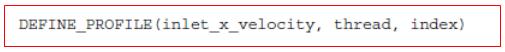
UDFs are implemented in FLUENT code as macros. The general format for a defined macros is the macro name that is define followed by a underscore with the udf name in parenthesis followed by a coma and then mentioning the variables that are to be passed, as shown in examples below.

The definitions for DEFINE macros are contained in the udf.h header file, hence it is not possible to have something else defined in the UDF that is outside the udf.h header file.

Letus say for example, if we want to define a customized velocity profile to a inlet we have to define something like as shown below.

Example :

The udf.h header file contains the following :

Definitions for DEFINE macros
#include compiler directives for C library function header files
Header files (for example, stdio.h) for other ANSYS FLUENT-supplied macros and functions

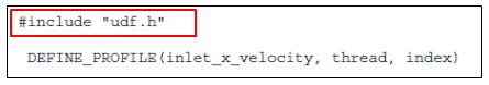
A UDF should begin with #include followed with "udf.h" followed by whichever macro to be used can be defined, shown below.

Compiling & Interpreting UDFs :

Now let us understand how a UDF is compiled or interpreted i.e. how a UDF is exactly included in the FLUENT software. The file containing the UDF can be either interpreted or compiled in FLUENT. The way in which the source code is compiled and the code that results from the compilation process is different for both cases. In compiled UDFs, the UDFs are built in same way as that the ANSYS FLUENT software itself is built, whereas in the interpreted UDFs the source code is compiled into a machine code that executes on an internal emulator whenever the UDF is invoked.

Let us now understand how UDFs are compiled. Basically they are compiled either by graphical user interphase (GUI) or the text user interphase (TUI) . In the case of GUI it is a two step process i.e. a window called compiled UDF flashes on the screen whenever we try to compile. The input it requires are :

Build a shared library object file from a source file
Load the shared library into FLUENT.

So to summarize we create a library file from our UDF C program, later we load the library file into FLUENT as if it is a part of FLUENT.

Now let us see how how interpreted UDF differ from compiled ones. This is a single step process, occuring at runtime only and involves use of interpreted UDFs dialog box.

Basically what happens when we interpret a UDF, is that the source code is compiled into an intermediate architecture machine code using a preprocessor. Now this machine code is executed on an internal emulator, or interpreter when the UDF is invoked . As an additional function is to be called during execution, it therefore incurs a reduction in performance.

Types of UDF :

As per the requirement the basic/ general practice goes as :

For small, straightforward functions we use interpreted UDFs
For complex functions that have high significant CPU requirement and require access to a shared library we use complied UDFs. Because compiled UDF is like a part of ANSYS FLUENT software itself.

Hooking UDFs into a problem setup :

We can either interpret or compile the UDF source file. Now the function contained in the interpreted code or shared library will appear in the dropdown list in dialogue boxes. We may choose this function to activate or "hook" our UDF in CFD model.

Eg : Now let us see an example of how UDF can be used.

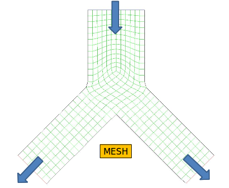
In this example a UDF is used to define a variable velocity profile to the inlet. The geometry is a very simple, i.e. flow is simply from top and gets divided into 2 outlets streams at left and right bottom. The image shown below is a representation of a hexahedral mesh used for the study.

First we will study a constant inlet velocity profile without the use of UDF, so the graph shown below is of a constant velocity profile i.e. 0.01 m/s in the negative Y axis.

After simulation the velocity contours display that the flow is taking some distance to develop the parabolic velocity profile (as seen below). This can be seen more clearly using the velocity vectors wherein we see straight profile at the inlet and after some time we see different color vectors in the same zone till the parabolic profile has been achieved.

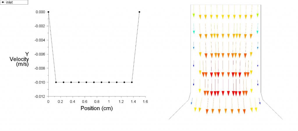
Plots in case of without a UDF

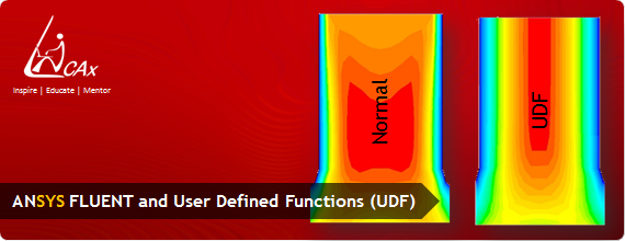
Now using the UDF, we can define a parabolic inlet as in the plot below; ranging from 0 to 0.01 m/s in negative Y axis direction, and the velocity contours of simulation has achieved the parabolic profile right at the very inlet; also proved using the velocity vector plot (shown below).

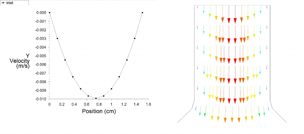
Plots in case of with-UDF

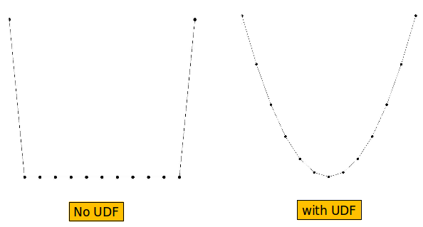
Comparative velocity profiles in the 2 cases (without & with UDF)

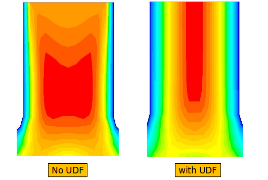
Comparative contour plots in the 2 cases (without & with UDF)

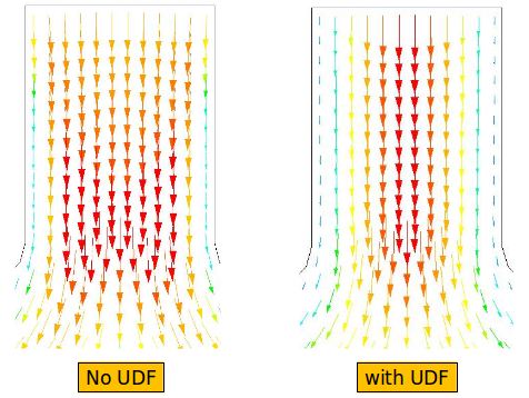
Comparative velocity vector plots in the 2 cases (without & with UDF)

Thus comparing both cases in detail, what we see is, without the use of UDF the velocity profile at the inlet was a straight line and along the length of the pipe it started developing the actual velocity profile. In order to achieve the actual velocity profile right at the inlet, we have to extend the inlet atleast till a length equal to or greater than the length the flow took to develop the profile. In this approach is where as with the use of UDF we could have the real velocity profile that is supposed to be at the inlet.

Software Demo :

A below video shows a demo in ANSYS FLUENT software.

{modal index.php/en/?option=com_content&view=article&id=118}

{/modal}

{modal index.php/en/?option=com_content&view=article&id=118}

{/modal}