Reviewing Governing Equations Of Fluid Dynamics

Reviewing Governing Equations of Fluid Dynamics

As all of CFD, in one form or the other is based on the fundamental governing equations of fluid dynamics i.e. the continuity, momentum and energy equations these are called as the equations speaking physics. They are the mathematical statements of the three physical principles that govern fluid dynamics, hence it becomes very important to derive and discuss these equations. The current blog is motivated to review the very basis of governing equations understanding their physical meaning before actually deriving them.

The primary objectives of studying or keeping oneself abreast with these equations being:

It is important for every student of CFD to be comfortable with these equations before embarking on any application of CFD to a particular problem.
For students from varied disciplines of engineering and experience these may serve as a source of enlightenment for novices and interesting for conversant.
As these governing equations can be obtained in various forms and the particular form of equation making little difference for a given algorithm the use of these equations in one form may lead to success and the alternate form into oscillations (wiggles) in numerical result or even instability.

Thus it is of vital importance to understand the meaning and significance of each of these equation, indeed of each term in these equation to properly interpret the CFD results obtained by numerically solving these equations.

Models of flow

The basic equations of fluid motion invariably follows the following three step philosophy:
1. Select appropriate fundamental physical principle from laws of physics such as:

Mass is conserved
F = ma, Newton’s II law
Energy is conserved

2. Apply these physical principles to a suitable model of the flow

3. Extract the mathematical equation which embody such physical principles.

Now while defining a suitable model of flow we know that a solid body is rather easy to see and define, on the other hand, a fluid is a ”squishy” substance that is hard to grab hold of. If a solid is in translational motion, the velocity of each part of the body is the same, on the other hand, if a fluid is in motion, the velocity may be different at each location in the fluid. For a continuum fluid, we need to construct one of the four models,discussed below to apply the fundamental physical principles.

Finite control volume

(Fig: 01; Image source: Computational Fluid Dynamics by John Anderson)

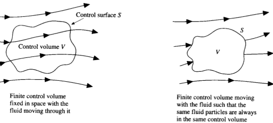
Let us imagine a closed volume; drawn within a finite region of the flow. This volume defines the control volume V ; a control surface S is defined as the closed surface that bounds the volume. The control volume may be fixed in space with the fluid moving through it as shown in figure 1 above (left hand side). As the fundamental physical principles are applied to the fluid inside the control volume and to the fluid crossing the control surface (if the control volume is fixed in space), therefore, instead of looking at the whole flow field at once, with the control volume model we limit our attention to just the fluid in the finite region of the volume itself. The fluid flow equations that we directly obtain by applying the fundamental physical principles to a finite control volume are in the integral form. These integral form of governing equations can be manipulated to indirectly obtain partial differential equations.

The equations so obtained from the finite control volume fixed in space, in either integral or partial differential form are called the conservation form of the governing equations. The equations obtained from the finite control volume moving with the fluid in either integral or partial differential form are called the non-conservation form of governing equations (image above at right hand side).

Infinitesimal fluid element

(Fig: 02; Image source: Computational Fluid Dynamics by John Anderson)

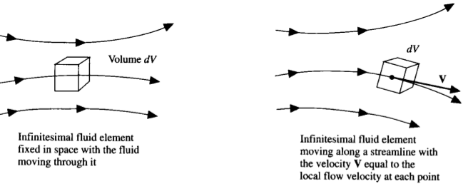
Let us imagine an infinitesimally small fluid element in the flow with a differential volume {tex}dV{/tex} . The fluid element is infinitesimal in the same sense as differential calculus; however it is large enough to contain a huge number of molecules so that it can be viewed as a continuous medium. The fluid element may be fixed in space with the fluid moving through it, alternatively may be moving along a streamline with a velocity vector {tex}\vec{V} {/tex} equal to the flow velocity at each point. Again instead of looking at the whole flow field at once, the fundamental physical principles are applied to just the infinitesimally small fluid element itself. This application leads directly to the fundamental equation in partial differential form. The particular partial differential equation obtained from the fluid element fixed in space are again the conservation form of the equation and the partial differential equation obtained directly from the moving fluid element are again called non-conservation form of the equation. Thus the governing equation can be expressed in the two general forms viz;
Thus the governing equation can be expressed in the two general forms viz;

conservation form
non-conservation form

Comments
Though, in general aerodynamic theory it is irrelevant whether we deal with the conservation or non-conservation forms of equation, it is certainly important in the case of CFD approach. The nomenclature used to distinguish these two forms (conservation versus nonconservation) has arisen primarily in the CFD literature. Through simple manipulation, one form can be obtained from the other.

The Substantial Derivative: Time rate of change following a moving fluid element

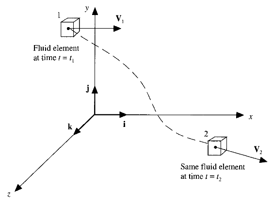
Before deriving the governing equation, we need to establish a notation which is common in aerodynamics , that of the substantial derivative, understanding its important physical meaning. Consider an infinitesimally small fluid element moving with the flow, through cartesian space. The unit vectors along the {tex}x{/tex},{tex}y{/tex} and {tex}z {/tex} axes are {tex}i{/tex}, {tex}j{/tex}, and {tex}k{/tex} respectively.

(Fig: 03; Image source: Computational Fluid Dynamics by John Anderson)

The vector field in this cartesian space is given by:
{tex} V = u{i} + v{j} + w{k} {/tex}

where the x,y and z components of velocity are given, respectively by:
{tex} u= u (x,y,z,t) \\ v= v (x,y,z,t) \\ w= w (x,y,z,t) {/tex}

Note: We are considering in general an unsteady flow, where {tex}u {/tex},{tex} v {/tex} and {tex}w{/tex} are functions of both space and time. In addition, the scalar density field is given by :

{tex} \rho = \rho(x,y,z,t) {/tex}

At time t, the fluid element is located at point 1, at this point and time the ρ of fluid element is:

{tex} \rho_1 = \rho(x_1,y_1,z_1,t_1) {/tex}

At a later time t2 , the same fluid element has moved to point 2 as shown in figure 2.

{tex} \rho_2 = \rho(x_2,y_2,z_2,t_2) {/tex}

Since {tex} \rho = \rho (x, y, z, t){/tex} we can expand this function in a Taylor series about point 1 as follows:

{tex} \rho_2 = \rho_1 + \left( \frac{\partial \rho}{\partial x} \right)_1 (x_2 - x_1) + \left(\frac{\partial \rho}{\partial y} \right)_1 (y_2 - y_1) + \left(\frac{\partial \rho}{\partial z} \right)_1 (z_2 - z_1) + \left(\frac{\partial \rho}{\partial t} \right)_1 (t_2 - t_1) + \mbox{higher order terms} {/tex} --(01)

Dividing both sides by {tex}(t_2 - t_1){/tex} and ignoring higher order terms

{tex} \frac{\rho_2 - \rho_1}{(t_2 - t_1)} = \left( \frac{\partial \rho}{\partial x} \right)_1 \left( \frac{x_2 - x_1}{t_2 - t_1}\right) + \left( \frac{\partial \rho}{\partial y} \right)_1 \left( \frac{y_2 - y_1}{t_2 - t_1}\right) + \left( \frac{\partial \rho}{\partial z} \right)_1 \left( \frac{z_2 - z_1}{t_2 - t_1}\right) + \left( \frac{\partial \rho}{\partial t} \right)_1 {/tex}

Note: The L.H.S is physically the average time rate of change in density of the fluid element as it moves from point 1 to point 2. Applying {tex}lim (t_2 \longrightarrow t_1){/tex}, it becomes;

{tex} \lim_{t_2 \to t_1} \left( \frac{\rho_2 - \rho_1}{t_2 - t_1}\right) = \frac{D\rho}{Dt} {/tex}

The term on the right side of the above equation (01) denotes the instantaneous time rate of change of {tex}\rho{/tex} of fluid element as it moves through space. Here our eyes are locked on the fluid element as it moves and we are watching the density of the element change as it moves through point {tex}1{/tex}. By definition {tex}\frac{D}{Dt}{/tex} is called the substantial derivative. This is different from {tex}\frac{\partial \rho}{\partial t}{/tex}, which is physically the time rate of change of {tex}\rho{/tex} at the fixed point {tex}1{/tex}. For {tex}\frac{\partial \rho}{\partial t}{/tex}, we fix our eyes on the stationary point {tex}1{/tex} and watch the density change due to transient fluctuations in the flow field.
Thus {tex}\frac{D \rho}{D t}{/tex} and {tex}\frac{\partial \rho}{\partial t}{/tex} are physically different
quantities:
Returning to equation (01):

{tex}\lim_{t_2 \to t_1} \left( \frac{x_2 - x_1} {t_2 - t_1} \right)_1 \equiv u {/tex}

{tex} \lim_{t_2 \to t_1} \left( \frac{y_2 - y_1} {t_2 - t_1} \right)_1 \equiv v {/tex}

{tex} \lim_{t_2 \to t_1} \left( \frac{z_2 - z_1} {t_2 - t_1} \right)_1 \equiv w {/tex}

Thus taking limit of equation (01), as {tex}t_2 \longrightarrow t_1{/tex} we get;

{tex} \frac{D\rho}{Dt} = u \frac{\partial \rho}{\partial t} + v \frac{\partial \rho}{\partial t} + w \frac{\partial \rho}{\partial t} + \frac{\partial \rho}{\partial t} {/tex} -------------(02)

From the above equation we can obtain an expression for the substantial derivative in cartesian coordinates:

{tex} \frac{D}{D t} \equiv \frac{\partial }{\partial t} + u \frac{\partial }{\partial x} + v \frac{\partial }{\partial t} + w \frac{\partial }{\partial t} {/tex} -------------(03)

Further more in cartesian coordinates the vector operator {tex}\nabla{/tex} is defines as:

{tex}\nabla \equiv i \frac{\partial }{\partial x} + j \frac{\partial }{\partial y} + k \frac{\partial }{\partial z} {/tex} -------------(04)

Further equation (03) can be written as;

{tex}\frac{D}{Dt} \equiv \frac{\partial }{\partial t} (V \cdot \nabla) {/tex} -------------(05)

Equation (05) represents a definition of the substantial derivative operator in vector notation, valid for any coordinate system.

Note: In above equation (05), {tex}\frac{\partial }{\partial t}{/tex}is the substantial derivative that is physically time rate of change following a moving fluid element, {tex}\frac{\partial }{\partial t}{/tex} is called the local derivative, which is physically the time rate of change at a fixed point; {tex} V \cdot \nabla{/tex}is called the convective derivative, which is physically the time rate of change due to the movement of fluid element from on location to another in the flow field where the flow properties are spatially different.

Again;

{tex}\frac{D T}{Dt} = \frac{\partial T}{\partial t} + (V \cdot \nabla) = \frac{\partial T}{\partial t} + u \frac{\partial T}{\partial x} + v \frac{\partial T}{\partial y} + w \frac{\partial T}{\partial z} {/tex} -------------(06)

Above equation (06) states physically that {tex}T{/tex} of the fluid element is changing as the element sweeps past a point in the flow because at that point the flow field {tex}T{/tex} itself may be fluctuating with time ({tex} \frac{\partial T}{\partial t} {/tex} local derivative term ) and because the fluid element is simply on its way to another point in the flow field when the temperature is different ({tex} V \cdot \nabla {/tex}, the convective derivative term).
We could have circumvented the above discussion as:

{tex}\rho = \rho(x,y,z,t){/tex}

Then by chain rule from differential calculus,

{tex}d\rho = \frac{\partial \rho}{\partial x} dx + \frac{\partial \rho}{\partial y} dy + \frac{\partial \rho}{\partial z} dz + \frac{\partial \rho}{\partial t} dt {/tex} ------- (07)

Dividing both sides by {tex}dt{/tex} ;

{tex}\frac{d\rho}{dt} = \frac{\partial \rho}{\partial t} + \frac{\partial \rho}{\partial x} \frac{dx}{dt} + \frac{\partial \rho}{\partial y} \frac{dy}{dt} + \frac{\partial \rho}{\partial z} \frac{dz}{dt} {/tex} ------- (08)

Since {tex}\frac{dx}{dt} = u, \frac{dy}{dt} = v, \frac{dz}{dt} = w{/tex}

{tex}\frac{d\rho}{dt} = \frac{\partial \rho}{\partial t} + u \frac{\partial \rho}{\partial x} + v \frac{\partial \rho}{\partial y} + w \frac{\partial \rho}{\partial z} {/tex} ------- (09)

Here {tex} \frac{d\rho}{dt}{/tex} and {tex}\frac{D\rho}{Dt}{/tex} are one and the same.

Divergence of velocity: Physical meaning

Divergence of velocity term: {tex} \nabla \cdot V {/tex}

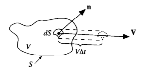
Consider a control volume moving with the fluid as shown in the figure below. This control volume is always made up of same fluid particles as it moves with the flow hence its mass is fixed and invariant with time. However its volume {tex}V{/tex} and control surface {tex} S {/tex} are changing with time as it moves to different regions of the flow where different values of {tex}\rho {/tex} exists i.e. this moving control volume of fixed mass is constantly increasing or decreasing its volume and is changing its shape, depending on the characteristics of the flow. At some instant in time it looks like below figure:

(Fig: 04; Image source: Computational Fluid Dynamics by John Anderson)

Consider an infinitesimal element of the surface {tex}dS{/tex} moving at the local velocity {tex}\vec{V}{/tex}, as in the above figure. The change in the volume of control volume, {tex}\Delta V{/tex}, due to just the movement of {tex}dS{/tex} over a time increment {tex}\Delta t{/tex} is from figure 4 equal to the volume of the long, thin cylinder with base area {tex}dS{/tex} and altitude {tex}(V \Delta t) \cdot \hat{n}{/tex} where {tex}\hat{n}{/tex} is a unit vector perpendicular to the surface at {tex}dS{/tex}.

{tex}\Delta V = [(\vec{V} \Delta t) \cdot n]dS = (V \Delta t)\cdot dS ~~~~~~(\mbox{where}: dS \equiv {/tex}n dS) ------- (10)

Over the time increment {tex}\Delta t{/tex}, the total change in volume of the whole control volume is equal to the summation of equation (10) over the total control surface. In the limit as {tex}dS \longrightarrow 0 {/tex}, the sum becomes the surface integral.

{tex}\int_s \int (V \Delta t) \cdot dS {/tex}

If this integral is divided by {tex}\Delta t{/tex}, the result is physically the time rate of change of the control volume, denoted by:

{tex}\frac{DV}{Dt} = \frac{1}{\Delta t} \int \int (\vec{V} \cdot \Delta t)\cdot dS \int_s \int \vec{V} \cdot dS {/tex} ------- (11)

Note: We have written the left hand side of equation (11) as the substantial derivative of {tex}V{/tex}, because we are dealing with the time rate of change of the control volume as the volume moves with the flow, and this is physically what we mean by the substantial derivative. Applying the divergence theorem from vector calculus to the right hand side of equation (11) we have:

{tex}\frac{DV}{Dt} = \int \int_V \int (\Delta \cdot V) dV {/tex} ------- (12)

Now let us imagine that the moving control volume in figure above is shrunk to a very small volume {tex}\delta V{/tex}, essentially becoming an infinitesimal moving fluid element as to the right of the figure 2, then;

{tex}\frac{D (\delta V)}{Dt} = \int \int_{\delta V} \int (\nabla \cdot V) dV {/tex} ------- (13)

Imagine that {tex}\delta V{/tex} is small enough such that {tex}\nabla \cdot V{/tex} is essentially the same value throughout {tex}\delta V{/tex}. Then the integral in equation (13) in the limit as {tex}\delta V{/tex} shrinks to zero, is given by, {tex}(V \Delta t)\cdot dV{/tex}. From equation (13), we have:

{tex} \frac{\delta V}{Dt} = (\nabla \cdot V) \delta V \\ \nabla \cdot V = \frac{1}{\delta V} \frac{D (\delta V)}{Dt} {/tex} ------- (14)

Note: The above equation (14) physically means that the time rate of change of the volume of a moving fluid element per unit volume.

In the further blogs I plan to come up with the detail derivations of these conservation equations for mass, momentum and energy in different forms separately.

References:

Disclaimer: The discussion in this blog is inspired and refereed from the well known books in CFD community viz; "Computational Fluid Dynamics" by JOHN ANDERSON & "An Introduction to Computational Fluid Dynamics" by H. K. VERSTEEG and W. MALALASEKERA. The author of the blog does not own or claim any copy right of the content discussed above and is purely intended only to serve as a guiding line for freshers in CFD, discussing the most respected works in the domain.

The Author

{module [317]}