No Meshing ! Its Meshless CFD
A most common complaint often cited by computational fluid dynamics practitioners is the generation of a good quality computational mesh and is estimated to be costing about 70% of the entire simulation cycle. Though much progress has been made in terms of algorithm accuracy and speed over the last three decades, generating grids step for complex, real world computations still remains the most time consuming and least reliable component of CFD simulation process. Meshless methods thus provide a viable alternative to grid-based flow computation as they are supposed to not require the conventional grid structure and thereby relieving the many issues specifically related to grid generation step. This blog shall provide you an introduction and update about the popular meshless methods available today.
So, what actually is a Mesh ?
Mesh or grid is defined as a discrete cell or elements into which the domain/ model is divided. All the flow variables & any other variables are solved at centres of these discrete cells. This entire process of breaking up a physical domain into smaller sub-domains (elements/ cells) is called as meshing or grid generation. These cells are grouped to form boundary zones and then boundary conditions are applied on these zones. Not only the generation of a good grid but also its maintenance is an onerous task that can dictate factors like:
- Rate of convergence
- Accuracy of result
- CPU time required.
Grid generation is performed manually by majority of practitioners though there have been recently additions of softwares with automated meshing features. Using the automated meshing approach the user has to provide basic inputs regarding cell size and zones to be meshed and the solver takes care of the grid generation. However this may not be feasible for all the cases as they hold limitations for complex geometries and hence a third approach was developed for CFD analysis called as "Meshless CFD".
What are Meshless method ?
A Meshless method is used to establish a system of algebraic equations for the whole problem domain without the use of a predefined mesh for the domain discretization. Nodes are scattered within the problem domain and also the set of nodes are scattered on the boundaries of the domain to represent (not discretize) the problem domain and its boundaries. No mesh implies that no information on the relationship between the nodes is required unlike in the conventional cases of finite volume or finite difference methods.
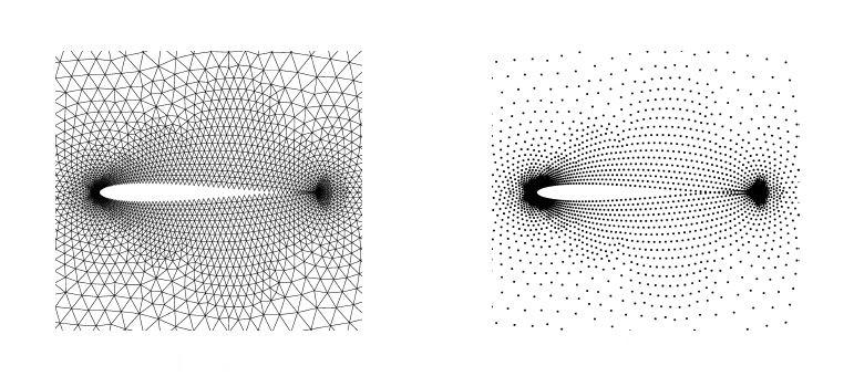 Image shows an airfoil which is meshed (Left) and the same airfoil which is surrounded by points (right) partial differential equations are solved on these points in meshless methods
Why go Meshless ?
Many existing numerical methods such as finite volume method, finite difference method requires mesh. In such a mesh, each point has a fixed number of predefined neighbors, and this connectivity between neighbors can be used to define mathematical operators like the derivative and using this information, equations are solved for the entire domain.
But in case of simulations, where material being simulated can move around or is subjected to large deformations (e.g. moving mesh problems), the connectivity of the mesh is difficult to maintain without introducing an error in simulation. Though in such cases the mesh can be recreated during simulation, ultimately leads to further addition of errors. Meshless methods are can act as a saviour for this problem.
Other advantages of meshless methods being:
- Time required for meshing is saved.
- Simulations on complex geometries can be done easily, as complex geometries are difficult to mesh and can take even few weeks for meshing.
- Human assistance required for meshing can be eliminated.
Different Meshless methods:
There are many meshless methods developed in recent years and we will have an overview of few of these methods without going into too much of technical specifications.
Smoothed Particle Hydrodynamics (SPH) :
SPH, is one of the oldest mesh-less method first used in astrophysics, and thereafter is now increasingly used in fluid flow studies. In this method node points are treated as physical particles with mass and density that can move around over time. Value of any property or its derivative is independent of values in adjacent particles in this method. Particles can be used in any order and doesn't matter if the particles move around or even exchange places.
The basic step of the method for domain discretization, field function approximation and numerical solution can be summarized as follows:
- The continuum is decomposed into a set of arbitrarily distributed particles with no connectivity (meshfree);
- The integral representation method is adopted for field function approximation;
- Particle approximation is introduced for converting integral representation into finite summation.
Radial Basis Functions (RBF) :
The development of RBFs into a mesh free method for solving partial differential equations arises from the recognition that a radial basis function interpolant can be smooth and accurate on any set of nodes in any dimension. RBF, is a function whose value depends only on distance from origin or any other specified point and are the means to approximate multivariable functions by linear combinations of terms based on a single univariable function (the radial basis function). These are usually applied to approximate functions or data which are only known at a finite number of points (or too difficult to evaluate otherwise).
Some commonly used types of RBF’s are
- Gaussian
- Multiquadric
- Inverse quadric
- Inverse multiquadric.
Finite Pointset Method (FPM):
FPM, is a particle method that uses Lagrangian approach and in this method the fluid is replaced by finite number of particles (points) that are non-stationary particles. These particles move with fluid velocities and carry fluid quantities like density, velocity, pressure. Similarly boundaries can be approximated by finite number of boundary particles and boundary conditions can be prescribed on them. As seen in SPH method, FPM also does not use rigid neighborhood list for a certain node/point (as in case of FVM). So all points/ particles are allowed to move and neighborhood list is recomputed at every time step.
This method is suitable for flows with complicated geometry, free surface flows, multiphase flows.
FPM method has some advantages over the widely used mesh free method, the SPH method. The main difficulty with SPH method is incorporation of boundary conditions. In FPM method this difficulty is taken care by using moving least square or least square approach in which the boundary conditions can be implemented in a natural way by just placing the particles on boundaries and prescribing boundary conditions on them.
Some Commercial Meshless CFD softwares
Let us get introduced to some commercial software available for meshless CFD.
XFlow:
It is one of the commercially available meshless software from Next Limit Dynamics. It uses Lattice Boltzmann equations and meshless particles based kinetic solver. The capabilities of XFlow are for solving following problems:
- Moving boundary problems
- Multiphase flows
- Fluid structure interactions
- Transient analysis
- Large eddy simulation
- Acoustics
- Non Newtonian flows
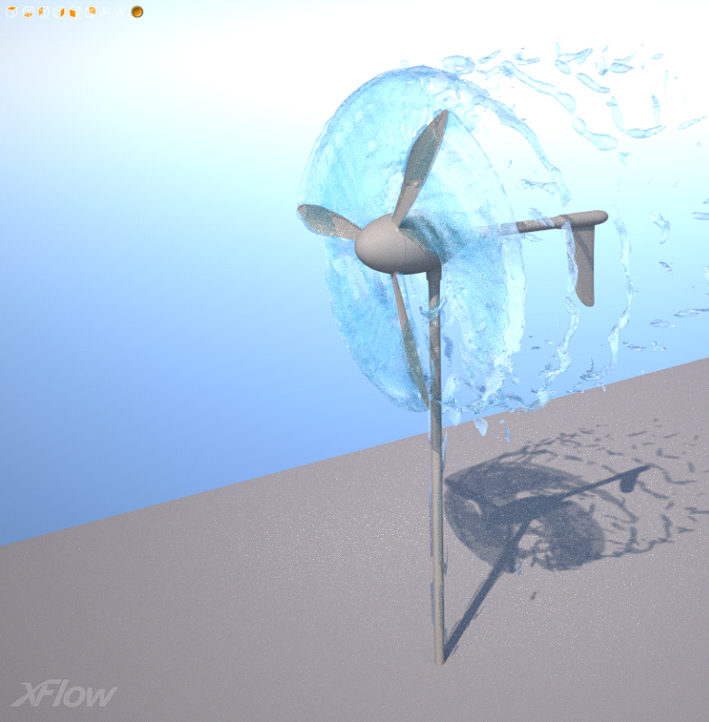
Wind turbine CFD simulation (Source: XFlow)
XFlow simulation can assess the efficiency of the turbine and predict loads on blades, wake turbulence intensity, or interference effects in wind farms. One can visit their website on http://www.xflow-cfd.com/ and can find many mesmerizing videos showing varied simulations.
NOGRID:
NOGRID, founded in the year 2006 and since then in use for CFD analysis. This meshless software in NOGRID uses Finite pointset method and Navier-Stokes equation to solve CFD problems. Special capabilities of this software are for:
- Multiphase flows
- Non-Newtonian flows
- Fluid structure interactions
NOGRID software is advantageous in situations where grid-based methods reach their limits due to the necessary remeshing. Using the fast and robust NOGRID solver the usual long modeling and computing times can be shortened substantially.
Animation shows velocity contours of CFD simulation of accelerated boat, created using NOGRID. (Source: NOGRID)
Animation shows velocity contours of CFD simulation of mixing tank, created using NOGRID. (Source: NOGRID)
One can visit this website to know more about this software: http://www.nogrid.com/index.php/en/
DualSPHysics:
This software is based on Smoothed-particle hydrodynamics method and is developed to study free-surface flow phenomena where Eulerian methods can be difficult to apply, such as waves or impact of dam-breaks on off-shore structures. It is an open source software product developed from collaborative effortsof researchers at the Johns Hopkins University (US), University of Vigo (Spain) and the University Of Manchester (UK). This software can also solve problems using GPU (Graphics processing unit). Following video shows an example of Floating-rigid body interactions and an example of visualization using DualSPHysics.
http://www.youtube.com/watch?v=ZK2ZWoWNnDY
http://www.youtube.com/watch?v=4IfgJJZcl_A
To know more about this software visit their website: http://dual.sphysics.org/
Algodoo:
Algodoo is developed by Algoryx Simulation AB. It is a 2 D simulation framework for education purpose which uses SPH method. It is very easy to use and can create good visualizations for education purpose and learn physics. It is a very good tool for science teachers and students.
This tool is not a like a high end CFD solver which gives you very accurate results. But it is a very good software for visualizing physics and doing many different simulations in very less time.
Along with fluid simulations Algodoo also supports some other physics like mechanics, optics. The video shows a various fluid simulations done using Algodoo and some of the simulations are done using other products of Algoryx.
http://www.youtube.com/watch?v=kzFam0UKFoA
Visit http://www.algodoo.com/ to know more and download the free software.
Meshless techniques save a lot of time and efforts required for meshing. Meshless CFD technique is flourishing and its future looks bright as it is a remedy on one of the biggest difficulties faced by every CFD engineer i.e “Meshing”.
References
- Classification and Overview of Meshfree Methods – by Thomas-Peter Fries, Hermann-Georg Matthies
- An Introduction to Meshfree Methods and Their Programming – by Gui-Rong Liu, Y. T. Gu
- Meshless methods for Computational Fluid Dynamics- Aaron John Katz
- http://www.xflow-cfd.com/
- http://www.nogrid.com/index.php/en/
- http://www.dual.sphysics.org/
- http://www.algodoo.com/
Further readings:
Interested readers can also get information from following books/ blogs :
- Meshfree Approximation Methods with MATLAB – by Gregory E. Fasshauer
- Progress on Meshless Methods – by A. J. M. Ferreira, E. J. Kansa, G. E. Fasshauer, V. M. A. Leitão
- USACM blog on Meshfree Methods
The Author
{module [317]}