Grid Generation for CFD Analysis of Turbomachinery
Though CFD has been widely used as a standard and well established engineering design analysis and optimization tool, the turbomachinery flow simulation still remains one of the challenges to handle. The typical reasons that make them so are the very complex nature of geometries and flow physics encountered in turbomachines. The following phenomena make turbomachinery flows extremely intricate and difficult to model for CFD simulation studies:

- Shear layer developing on curved surfaces
- Have separated flows due to shock and boundary layer interactions (in transonic case) or corner separation during stall
- Involve swirling flows and vortices
- Interacting boundary layer (between blade surface and casing and end wall boundary layers)
In the complete CFD analysis of turbomachines, Grid generation becomes a very challenging task. This is mainly due to the geometries that are often complicated with twisted blades of different curvatures at different radii. This adds to the stringent meshing requirements to capture the above mentioned flow features. Having already gone through the CAD cleanup for CFD analysis of turbomachines in our earlier blog CAD Repair for CFD Analysis of Turbomachinery, we shall now have an overview of the best practices followed in industry for grid generation of a rotating machine with a software demo video.
Grid Generation:
Process of discretization of a fluid domain into smaller volumes made up of quad/hex, tri/tet, and prism elements is called grid generation. Mesh generation for a turbo/ rotating machines involves the following steps:
1. Choice of Mesh/Grid Type :
Fluid flow analysis in turbo-machinery demands a high quality hexahedral mesh to simulate the flow-path. Structured hexahedral mesh is created using Multi-block method and is preferred over unstructured tetrahedral mesh for the following reasons,
- Relatively less cell count needed to resolve geometry
- Provides more accuracy
- Easy boundary layer resolution
- Can have relatively large aspect ratio than unstructured cells
A structured hexahedral mesh provides lower cell count and reduced numerical error if the mesh is aligned with the flow. On the downside cell quality suffers with increased geometric complexity. So, after CAD clean-up, the feasibility of creating a structured multi-block hexahedral mesh for the geometry should be studied.
For more complex or odd geometries, possibility of hexahedral mesh becomes thin and an unstructured tetrahedral mesh is preferred over hexahedral mesh. In such cases, along with tetrahedrons, generating good quality prism cells on the wall surfaces becomes necessary, to resolve boundary layer and to maintain first cell height thereby wall Y+ value that a turbulence model demands.
In some cases, a hybrid mesh is generated i.e., hexahedral mesh is generated in the impeller (rotating fluid) region and a tetrahedral + prism mesh is created in the volute/casing (stationary fluid zone) region. In such cases, the interface may have a non-conformal mesh connectivity.
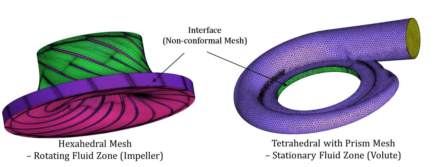
Usually, a multi-block hexahedral mesh approach is used for axial flow machines and a hybrid mesh approach is used for radial/centrifugal and mixed flow machines. So, the choice of mesh depends on the complexity of the geometry and nature of flow physics we are interested to study.
2. Periodic Meshing :
To reduce the time, efforts and complexity of meshing the rotational periodicity of the impeller geometry is taken advantage. Axial machines and rotating fluid zone of radial & mixed flow machines are meshed using this approach. Choosing a single periodic flow passage is the first step in this approach. The periodic angle of the flow passage is decided by the number of vanes/blades present.
Periodic angle or Angle of Rotational Periodicity = 360° / number of blades
Example :
- For a radial turbine with 16 blades, Angle of rotational periodicity = 360° / 16 = 22.5° (single blade passage)
- For a pump with 4 blades, Angle of rotational periodicity = 360° / 4 = 90° (single blade passage)
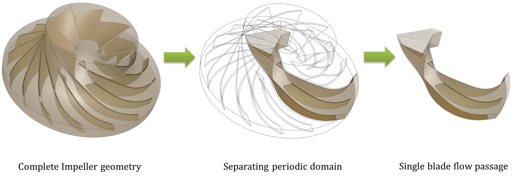
This periodic geometric sector can be chosen in two different ways.
- Flow passage between two blades (suction side of first blade to the pressure side of next blade)
- To have one complete blade inside the periodic flow passage
There are two different scenarios based on the flow physics. If the flow physics is also periodic (most axial flow machines), the mesh is generated only for a single blade fluid passage (theta), regardless of the number of blades and is directly used for simulation.
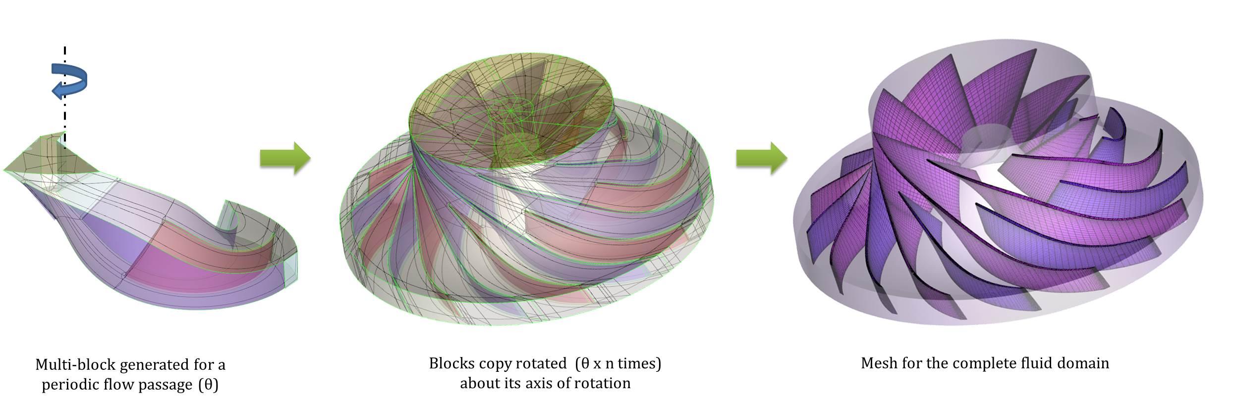
But if the flow physics is not periodic (radial & mixed flow machines with volute), the mesh is generated for the single periodic flow passage / sector and is copy rotated to get mesh for the complete geometry (360°). Meshing software provides an option for periodic meshing to ensure both sides of periodic passage has same number of nodes and same node location with a rotational offset of theta.
3. Mesh Size/Count :
Mesh size or count is nothing but the total number of cells used to fill the flow domain. The required mesh size depends on the complexity of the geometric features and the purpose of simulation. The number of nodes or cells assigned should be sufficient enough,
- To resolve the geometry
- To capture the flow physics
As a thumb rule, following cell counts are used:
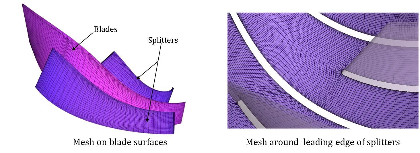
- Blade surfaces (stream wise) – 100 to 120 cells
- Blade to blade direction (radial) – 50 to 60 cells
- Hub to shroud direction – 30 to 40 cells
- Around leading and trailing edges – 15 to 30 cells
Thermal simulation/Conjugate heat transfer simulation requires a refined surface mesh to obtain realistic heat flux values at the fluid-solid interface.
4. Boundary Layer Resolution :
Cell count normal to the wall depends on the level of boundary layer resolution and the first cell height required for the wall function being used.
For design iterations, a wall function approach is sufficient. This requires a wall Y+ value between 20 to 200 for the first cell. The outer limit of the Y+ depends on the actual Reynolds number. For a low Re flow, keep the maximum wall Y+ value as low as possible. Boundary layer region should have 8 to 10 cells in wall normal direction.
For more accurate solution where loss prediction is very important, a wall treatment approach is used. This requires a wall Y+ value less than 1 for the first cell. Boundary layer region should have 15 to 30 cells in wall normal direction.
5. Mesh Quality :
The final mesh is smoothened to ensure quality criteria required by the CFD solver. This is an important step as the quality of mesh has an impact on rate of convergence, solution accuracy and CPU time required.
In the boundary layer region, high grid resolution with a cell expansion ratio of 20 to 25% is maintained. In regions other than boundary, the expansion ratio can go from 30 to 50% where the cell direction does not change suddenly.
A short video with mesh generation for the periodic sector and its copy rotated to create mesh for the entire geometry using ANSYS ICEM CFD software is demonstrated.
|
{modal index.php/en/?option=com_content&view=article&id=128}
 {/modal} {/modal}
{modal index.php/en/?option=com_content&view=article&id=128}
 {/modal} {/modal} |
Further in our next blog we shall try to explore about the different solver models used to simulate turbomachinery flows.
References :
- http://en.wikipedia.org/wiki/Turbomachinery
- Mod-01 Lec-38 CFD for Turbomachinery: Grid Generation, Boundary Conditions for Flow Analysis, NPTEL, Turbomachinery Aerodynamics by Prof. Bhaskar Roy,Prof. A M Pradeep, Department of Aerospace Engineering, IIT Bombay.
- MIT course ware/multi stage axial compressor-http://web.mit.edu/16.unified/www/FALL/thermodynamics/notes/node91.html
- An Introduction to Energy Conversion: Turbomachinery, Volume 3 by V. Kadambi, Manohar Prasad.
The Author
{module [317]}