Good Looking Mesh May Not Always be Good for the Simulation
As a computational geometry developer I have worked on several meshing software development projects. Every time mesh quality has become focal point. As matter of fact this becomes conflicting topic between the various teams due to the difference of opinion in engineering community.
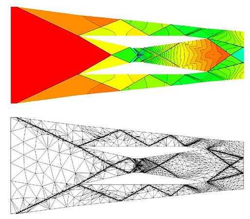
For example let’s consider you are doing FEA and CFD analysis of an aircraft wing. FEA simulation is performed to predict stresses and deflection whereas CFD simulation is performed for predicting lift & drag. Following image shows mesh used for FEA and CFD simulation of a wing.
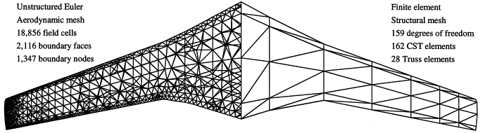
Looking at this image one can say “Good mesh for FEA can be a bad mesh for CFD”. But then that would be a too simplistic judgment !!!
One thing is sure one cannot generalize a good mesh purely based on geometric parameter. Mesh quality is very much dependent on the purpose (numerical simulation) for which one want to use it. To elaborate this point let’s consider CFD simulation of aircraft wing.
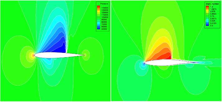
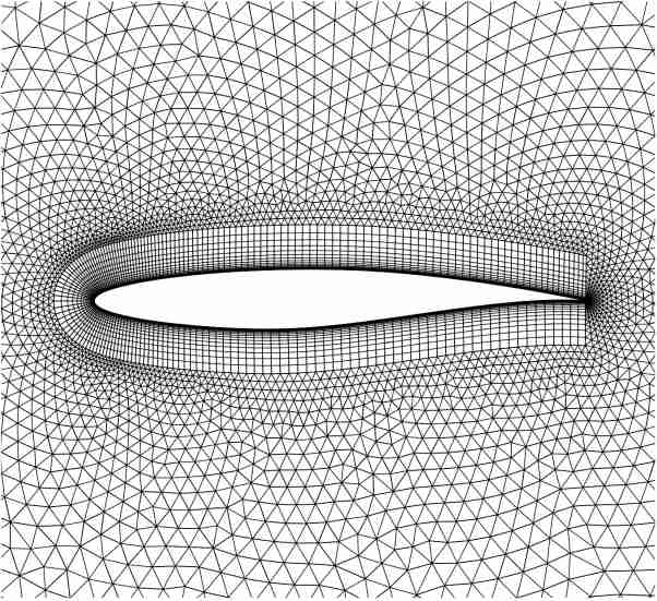
Typically in aerodynamic, scientist performs Euler simulation or Navier stokes simulation. In above picture left side image is from Euler simulation and right side image is from Navier stokes simulation. Euler simulation provides results very fast but does not consider viscosity effects in simulation. Therefore mesh wrapped around the wing is typically suitable for the Euler simulation. This type of mesh configuration is also known as O topology mesh.
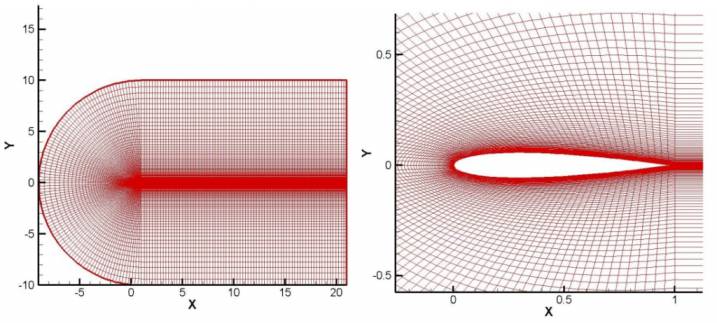
But if you want to take viscosity into account then one need to perform Navier stokes simulation. For Navier stokes (NS) simulation you need a dense mesh near the wing tip and in the wake region. Following figure shows mesh suitable for NS simulation. NS simulation takes more time to converge as compared to Euler simulation, but preferred due to the accuracy.
Therefore generally a novice CAE user makes mistake in defining quality mesh based on few parameters. Mesh which has all good looking equilateral triangles or square quadrilateral is good mesh!
But that may not be the true for every case. For example let’s look at ugly looking anisotropic mesh. Although this has lot of skewed elements it provides much better results where there is sudden change in property.
(Ref: Database of Polish Centres of Excellence)
Rules of Quality Mesh
Finite element methods and computational fluid dynamics applications place constraints on both the shapes and sizes of the mesh elements. There are several reasons for these constrains. The main purpose of mesh is to get fast and accurate solution for the simulation problem. Following simple rules are generally used by CAE engineers to quantify good mesh.
- The greater the rate of convergence, the better is the mesh quality : It means that the correct solution has been achieved faster. An inferior mesh quality may leave out certain important phenomenon such as the boundary layer that occurs in fluid flow. In this case the solution may not converge or the rate of convergence will be too less.
- A better mesh quality guarantees a more accurate solution : For improving the mesh quality for accurate solution, one may need to refine the mesh at certain areas of the geometry where the gradient of the field whose solution is sought is high. Also this means that, if a mesh is not sufficiently refined, the accuracy of the solution is more limited. Thus the required accuracy in turn dictates the mesh quality.
- CPU time is a necessary yet an undesirable factor : For a highly refined mesh, where the number of cells per unit area is maximum the CPU time required will be relatively large. In general, if the CPU time taken is more it indicates that the solution that is being generated will be of good accuracy. However, for the solution of given accuracy and rate of convergence, greater CPU time required indicates an inferior mesh quality.
I think above set of rules set up good ground rules for mesh quality for numerical simulation.
How bad meshes can affect your numerical solver?
There are several reasons because of which numerical solver insist use of good quality mesh. Following four are the main concerns:
- First, large angles (near 180°) can cause large interpolation errors. In the finite element method, these errors induce a large discretization error the difference between the computed approximation and the true solution of the PDE.
- Second, small angles (near 0°) can cause the stiffness matrices associated with the finite element method to be ill conditioned. Small angles do not harm interpolation accuracy, and many applications can tolerate them.
- Third, smaller elements offer more accuracy, but cost more computationally. Small element also can cause floating point errors.
- Fourth, small or skinny elements can induce instability in the explicit time integration methods employed by many time dependent physical simulations.
The first constraint forbids large angles, including large plane angles in triangles and large dihedral angles in tetrahedra. Most applications of triangulations use them to interpolate a multivariate function whose true value might or might not be known.
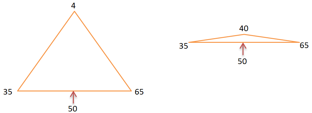
For example let’s consider triangle shown in above diagram is used to interpolate the temperature property. Temperature at bottom edge vertices are 35 and 65. Therefore temperature interpolated at the center of edge is 50. As the angle at the upper vertex start to approach 180 degree, the interpolated point with value 50 become close to top vertex with value 40. This increases the interpolated gradient by large magnitude and may be far away from true value.
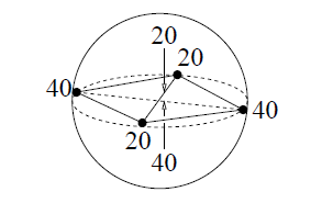
This error also occurs in sliver tetrahedra as shown in figure. A sliver is a tetrahedron that is nearly flat even though none of its edges is much shorter than the others. A typical sliver is formed by uniformly spacing its four vertices around the equator of a sphere, then perturbing one of the vertices just off the equator so that the sliver has some (but not much) volume.
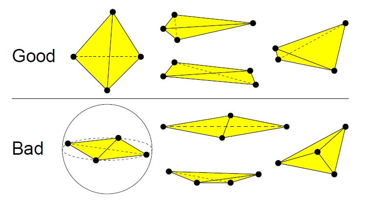
Good and Bad tetrahedra for interpolation
How does mesh quality impact my solver ?
The main point here is that small angles can cause poor conditioning, that the relationship can be quantified in a way useful for comparing differently shaped elements. To elaborate further on poor conditioning of matrices: some matrices are very sensitive to small changes in input data. The extent of this sensitivity is measured by the condition number. The definition of condition number is: consider all small changes δA and δb in A and b and the resulting change, δx, in the solution x. Then:
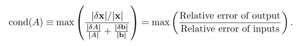
Put another way, changes in the input data get multiplied by the condition number to produce changes in the outputs. Thus a high condition number is bad. It implies that small errors in the input can cause large errors in the output.
Does mesh quality impact changes based on iterative methods or direct methods used in Solver?
The systems of linear equations constructed by finite element discretization are solved using either iterative methods or direct methods. The speed of iterative methods, such as the Jacobi and conjugate gradient methods depends in part on the conditioning of the global stiffness matrix: a larger condition number implies slower performance. Direct solvers rarely vary as much in their running time, but the solutions they produce can be inaccurate due to round off error in floating-point computations, and the size of the round off error is roughly proportional to the condition number of the stiffness matrix. As a rule of thumb, Gaussian elimination loses one decimal digit of accuracy for every digit in the integer part of the condition number. These errors can be countered by using higher-precision floating-point numbers.
Conditioning of global stiffness matrix
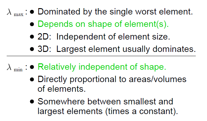
Time-dependent PDEs are usually solved with the help of standard integration methods for computing approximate solutions of ordinary differential equations. The stability of explicit time integration methods is linked to the largest eigenvalue of a matrix related to the stiffness matrix. This eigenvalue is related to the sizes and shapes of the elements.
Time-dependent PDEs are usually treated by the use of a finite element method to discretize the spatial. Dimensions only, yielding a system of time-dependent coupled ordinary differential equations (ODEs). The solution to this system of equations is approximated by means of any of a variety of standard numerical methods for integrating ODEs. Numerical time integration methods discretize time by dividing it into discrete time steps. Most time integration methods can be categorized as implicit or explicit. When implicit methods (such as centered differencing or backward differencing) are chosen, it is usually because they have the advantage of unconditional stability: numerical errors, which are introduced by the approximation or by floating-point round off error, are not amplified as time passes. By contrast, explicit methods are stable only if each time step is sufficiently small. The largest permissible time step is related to the stiffness matrix.
In summary, a good mesh is the one which suffice its purpose that is solving the physics.
Reference
- Delaunay Mesh Generation (Chapman & Hall/CRC Computer & Information Science Series) Siu-Wing Cheng , Tamal K. Dey, Jonathan Shewchuk (Highly recommended)
- What is a Good Linear Finite Element? Jonathan Richard Shewchuk
The Author
{module [313]}