Basics Of Y Plus Boundary Layer And Wall Function In Turbulent Flows

Basics of Y Plus, Boundary Layer and Wall Function in Turbulent Flows

Before getting into the details of the turbulent models let us discuss an important concept known as $y^{+}$ and know how it is related to turbulence modeling, mesh generation process and how it is going to affect the CFD end result. It is important to know about the concept of wall $y^{+}$ or in general how the flow behaves near the wall, to consider the effects near the wall as it is the basis on which choice of the turbulence model is governed.

The behaviour of the flow near the wall is a complicated phenomenon and to distinguish the different regions near the wall the concept of wall $y^{+}$ has been formulated. Thus $y^{+}$ is a dimensionless quantity, and is distance from the wall measured in terms of viscous lengths.

Why do we need $y^{+}$ ?

One of the reasons for the need of $y^{+}$ is to distinguish different regions near the wall or in the viscous region, however how exactly it helps in turbulence modelling or in general CFD modelling need to be well understood. Let us try to understand this with an example. A fisherman uses fishing net, a grid kind of structure to trap the fishes. If he is trying to catch medium to big sized fishes the grids in the net he uses is somewhat big, but if he is trying to trap even small sized fishes then the grid size of the net should be small enough to capture them. In this case even the large fishes are also captured. Similarly coming back to our case if we intend to resolve the effects near the wall i.e., in the viscous sub layer then the size of the mesh size should be small and dense enough near the wall so that almost all the effects are captured. But in some cases if the wall effects are negligible then there is option of including semi-empirical formulae to bridge between the viscosity affected region and fully turbulent region and in this case the mesh need not to be dense or small near the wall i.e., coarse mesh would work.

Considering the first case i.e., near wall modelling it is well-known that the mesh size should be small enough, however then the question follows is how small ? Thus, here comes the concept of $y^{+}$ , and based on the $y^{+}$ value the first cell height can be calculated. The near wall region is meshed using the calculated first cell height value with gradual growth in the mesh so that the effects are captured and avoiding overall heavy mesh count. Let us now look at the $y^{+}$ concept i.e., what exactly it is ? What is its mathematical form? How different regions are distinguished in viscous sub layer based on different $y^{+}$ values? But before that let us refresh the concept of boundary layer especially turbulent boundary layer.

Boundary layer theory

In a flow bounded by a wall, different scales and physical processes are dominant in the inner portion near the wall, and the outer portion approaching the free stream. These layers are typically known as the inner and outer layers. Considering the flow over a smooth flat plate the boundary layer can be distinguished into two types namely laminar boundary layer and turbulent boundary layer. Since we are dealing with the turbulent boundary layer let us not get into the laminar boundary layer. Typical boundary layer structure over a flat plate is shown below. In between the laminar and turbulent boundary layer there lies a transition region. Typically for flow over a flat plate the transition usually occurs around $Re\approx 5 \times 10^{5}$ .

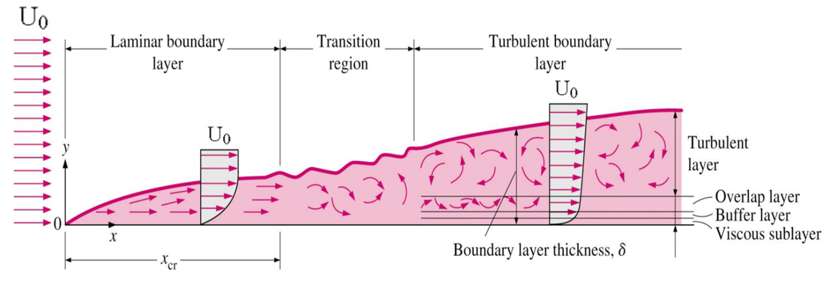
(Reference: Y. Cengel, Fluid Mechanics: Fundamentals and Applications)

Since we have discussed about the turbulent flow characteristics in the previous blog Introduction to Turbulence, we shall not get into it and directly discuss the turbulent boundary layer. From the above figure it can be seen that in turbulent boundary layer region flow near the wall has been analyzed in terms of three layers:

The inner layer, or sublayer, where viscous shear dominates
The outer layer, or defect layer, where large scale turbulent eddy shear dominates
The overlap layer, or log layer, where velocity profiles exhibit a logarithmic variation

A still clear image of the above is shown below:

Source: Applied Computational Fluid Dynamics by André Bakker

where $U_{0}$ is the free stream velocity and $\delta$ is the boundary layer thickness, $y$ is the vertical distance measured from the wall.

Turbulent boundary layers are usually described in terms of several non-dimensional parameters. The boundary layer thickness, $\delta$ is the distance from the wall at which viscous effects become negligible and represents the edge of the boundary layer.

Now let us discuss more about the above said regions. Owing to the presence of the solid boundary the flow behavior and turbulent structure are considerably different from free turbulent flows. Dimensional analysis has greatly assisted in correlating the experimental data. In turbulent thin layer flows a Reynolds number based on length scale $L$ in the flow direction $Re_{L}$ is always very large. This implies that inertia forces are greater than viscous forces at these scales. If we consider Reynolds number on a distance $y$ away from the wall $Re_{y}=U_{0}y/u$ , we see that if the value of $y$ is of the order of $Re_{y}=U_{0}L$ the above argument holds well. Inertia force dominates far away from the wall. As $y$ also decreases to zero. Just before $y$ reaches zero there will be a range of values of $y$ for which $Re_{y}$ is of the order 1. At this distance from the wall and closer, the viscous forces will be equal in the order of magnitude to the inertia forces or large. To conclude, in flows along solid boundaries there is usually substantial region of inertia dominated flow far away from the wall and a thin layer within which viscous effects are important.

Near to the wall the flow is influenced by the viscous effects and independent of free stream parameters. However the mean flow velocity depends on by $y$ (distance from the wall), $\rho$ (fluid density), $\mu$ (viscosity) and $tau_{w}$ (wall shear stress).

Thus: $U_{0}= f (y, \rho, \mu, \tau_{w})$

Linear sub-layer

At the solid surface the fluid is stationary and the turbulent eddying motion must also stop very close to the wall. The fluid very close to the wall is dominated by viscous shear in absence of the turbulent shear stress effects ( $y^{+}<5$ ) and it can be assumed that the shear stress is almost equal to the wall shear stress $\tau_{w}$ throughout the layer.

Thus we have: $\\tau (y) = \mu \frac{\partial U}{\partial y} \approx \tau_{w}$

Applying boundary conditions and manipulations we obtain:

$u^{+} = y^{+}$

Now as can be seen from the expression above to be a linear, the fluid layer adjacent to the wall is called as linear sub layer.

Log-law layer

At some distance from the wall and outside the viscous sub-layer $(30<y^{+}<500)$ a region exists where viscous and turbulent effects are both important. Within this inner region the shear stress is assumed to be constant and equal to wall shear stress and varying gradually with distance from the wall. The relationship between $y^{+}$ and $u^{+}$ in the region is given as:

$u^{+} = \frac{1}{k} ln y^{+} + B = \frac{1}{k} ln E y^{+}$

where $k$ , $B$ and $E$ are constants whose values are found from measurements.

As the relationship between $y^{+}$ and $u^{+}$ is logarithmic, the above expression is known as log-law and the layer where $y^{+}$ takes the values between 30 and 500 is known as log-law layer.

Outer layer

According to experimental studies it was found that the log-law is valid in the range $0.2 < \frac{y}{\delta}<0.2$ and for higher values of $y$ the defect law is referred, whereas in the overlap region the log-law and velocity defect law (law of wake) are equal. Tennekes and Lumley (1972) proposed the following logarithmic law for identifying the matched overlap region.

$\frac{U_{max} - U}{u_{\tau}} = \frac{1}{k} ln \frac{y}{\delta} + A$

Buffer layer

In the buffer layer, between 5 wall units and 30 wall units, neither law holds, such that:
For $5<y^{+}<30$
With the largest variation from either law occurring approximately where the two equations intercept, at $y^{+}=11$ . That is, before 11 wall units the linear approximation is more accurate and after 11 wall units the logarithmic approximation should be used, though neither are relatively accurate at 11 wall units.
Schematic diagram of the above laws or in general law of wall is shown below:

Velocity profiles in turbulent wall flow

The near-wall modeling significantly impacts the fidelity of numerical solutions, inasmuch as walls are the main source of mean vorticity and turbulence. After all, it is in the near-wall region that the solution variables have large gradients, and the momentum and other scalar transports occur most vigorously. Therefore, accurate representation of the flow in the near-wall region determines successful predictions of wall-bounded turbulent flows.

The k-ε models, the RSM, and the LES model are primarily valid for turbulent core flows (i.e., regions somewhat far from walls). Consideration therefore needs to be given as to how to make these models suitable for wall-bounded flows. The Spalart-Allmaras and $k-\omega$ models were designed to be applied throughout the boundary layer, provided that the near-wall mesh resolution is sufficient.

The two approaches are schematically shown below:

Reference: Near-Wall Treatments in ANSYS FLUENT

In most high-Reynolds-number flows, the wall function approach substantially saves computational resources, because the viscosity-affected near-wall region, in which the solution variables change most rapidly, does not need to be resolved. The wall function approach is popular because it is economical, robust, and reasonably accurate. It is a practical option for the near-wall treatments for industrial flow simulations.

The wall function approach, however, is inadequate in situations where the low-Reynolds-number effects are pervasive in the flow domain in question, and the hypothesis underlying the wall functions cease to be valid. Such situations require near-wall models that are valid in the viscosity-affected region and accordingly integrable all the way to the wall.

From above discussion it is clear that the placement of the first node in our near-wall inflation mesh is very important.

(Reference: Leap CFD)

From the above image we need to be careful to ensure that our $y^{+}$ values are not so large that the first node falls outside the boundary layer region. If this happens, then the Wall Functions used by our turbulence model may incorrectly calculate the flow properties at this first calculation point which will introduce errors into our pressure drop and velocity results.

Let us see how to calculate first cell height. Firstly, we should calculate the Reynolds number for our model based on the characteristic scales of our geometry.

From the definition of $y^{+}$ , we know: $y^{+}=\frac{\rho U_{\tau} \Delta y}{\mu}$
where $U_{\tau}$ is shear velocity. The target $y^{+}$ value and fluid properties are known a priori, so we need to calculate the frictional velocity as given above.
The wall shear stress, $\tau_{w}$ can be calculated from skin friction coefficient, $\C_{f}$ is such that: $\\tau_{w} = \frac{1}{2}C_{f} \rho U_{0}^{2}$

Thus to calculate we need to know, there are empirical formulae to calculate $\C_{f}$ which are given as:

For internal flows - $C_{f} = 0.079 * Re^{-0.25}$
For external flows - $C_{f} = 0.058 * Re^{-0.2}$

Thus with all these inputs we can insert the values in the above equation to calculate $\Delta y$ .

When considering simple flows and simple geometry, we might find this correlation to be highly accurate. However, when considering complex geometry, refinement in the boundary layer may be required to ensure the desired $y^{+}$ value is achieved. In such cases re-mesh has to be done or else mesh adaption techniques has to be used to achieve the required value across the entire model.
Thus we have learnt that the wall function approach and $y^{+}$ value required is determined by the flow behavior and the turbulence model being used. If we have an attached flow, then generally we can use a Wall Function approach, which means a larger initial $y^{+}$ value, smaller overall mesh count and faster run times. If one expects to have flow separation and knows that the accurate prediction of the separation point will be having an impact on the result, then he would be advised to resolve the boundary layer all the way to the wall with a finer mesh. Unfortunately, as the $y^{+}$ value is dependent on the local fluid velocity which varies across the wall significantly for most industrial flow applications, it is not possible to know the exact $y^{+}$ prior to running an initial simulation. Hence, it is important for one to get into the habit of checking the $y^{+}$ values as part of his normal post-processing so that one can make sure to fall in the valid range for the flow physics and turbulence model selection.

{module [315]}

References

The Authors

{module [311]}

{module [312]}